How Out-of-Level Testing Affects the Psychometric Quality of Test Scores

Out-of-Level Testing Project Report 2

Published by the National Center on Educational Outcomes

Prepared by John Bielinski, Martha Thurlow, Jane Minnema, and Jim Scott

August 2000

This document has been archived by NCEO because some of the information it contains may be out of date.

Bielinksi, J., Thurlow, M., Minnema, J, & Scott., J (2000). How out-of-level testing affects the psychometric quality of test scores    (Out-of-Level Testing Project Report 2 ). Minneapolis, MN: University of Minnesota, National Center on Educational Outcomes. Retrieved [today's date], from the World Wide Web: http://cehd.umn.edu/NCEO/OnlinePubs/OOLT2.html

Executive Summary

This report is a review and analysis of the psychometric literature on the topic of out-of-level testing. It reveals many significant concerns about the research that has been conducted, and identifies additional research needs. Much of the research on out-of-level testing was conducted in the 1970s and early 1980s. That research focused on the impact that out-of-level testing had on test performance and test score reliability. A very popular index of reliability was the percent of scores at or below chance level. This emphasis on chance level scoring has detracted from the field’s understanding of how out-of-level testing actually works to affect score reliability. The studies said nothing about the more important concept of measurement error. Furthermore, there was little discussion about the detrimental effects of translating scores from an out-of-level test back into the scale of the in-level test.

The literature indicates that the benefit of out-of-level testing is that it is a cost-effective method for increasing the precision with which low performing students’ ability is measured. However, an unreported downside is that the process by which scores on out-of-level testing are converted back into the scale of the in-level test reduces measurement precision. Further, it has not been demonstrated that more precision is gained than is lost.

In this report we use basic concepts of psychometric theory as a framework to describe how out-of-level testing affects test score quality. We emphasize the link between test difficulty, individual ability, and measurement error. We define the concepts of measurement precision and accuracy and relate them to the concepts of reliability and validity to help the reader better understand how out-of-level testing affects each. We then discuss the neglected topic of the measurement error that is introduced by the equating process used to translate out-of-level test scores onto the in-level scale.

The dramatic increase in the use of out-of-level testing that appears to be taking place across the United States today certainly is not justified by the findings of our analysis. Furthermore, the application of an approach developed within a norm-referenced testing context seems to be inappropriate and untested in the current context of standards-based assessments.

Out-of-level testing refers to the practice of using a level of a test other than the test taken by most of the students in a student’s current grade level (Thurlow, Elliott, & Ysseldyke, 1999). This practice has a long history of use, but most notable is its use in Title I testing in the 1960s and 1970s (Minnema, Thurlow, Bielinski, & Scott, 2000). Recently, out-of-level testing appears to be gaining popularity in state and district testing used for school accountability purposes (Thurlow et al., 1999). This increase in popularity has occurred, for the most part, without an analysis of the psychometric issues that surround out-of-level testing. Yet, the psychometric arguments for out-of-level testing are used as justification for its appropriateness.

Among the psychometric concepts central to out-of-level testing are "accuracy," "precision," and "vertical equating." It is important to examine each of these concepts carefully, especially when one considers that out-of-level testing may be widely recommended for use with students with disabilities as they participate in state and local educational accountability systems – an arena outside that for which out-of-level testing was originally considered (Elliott & Thurlow, 1999; Thurlow et al., 1999).

The purpose of this report is to clarify the psychometric basis for out-of-level testing. Concepts such as chance level scoring, which serves as a proxy for the more central concept of measurement error, will be replaced by measurement theory that shows the link between test difficulty, person ability, and measurement error. We attempt to explain relevant advanced measurement concepts so they are understood by a wider audience than psychometricians.

We begin by making clear the distinction between accuracy and precision. Following this is an illustration of the ways in which out-of-level testing may improve measurement precision for low scoring examinees, and the conditions under which this is so. These are important to understand because the conditions limit the usefulness of out-of-level testing, particularly for standards-based assessments. Following this, we review the role that vertical equating plays in translating scores from an out-of-level test to the grade-level test. Here we note the added measurement error introduced to test scores through vertical equating. Finally, we conclude with a review of empirical studies in which students were given both a grade level and an out-of-level test.

This report is not intended to be a synthesis of the research on out-of-level testing, nor is it intended to be a policy guide (see Thurlow, Elliott, & Ysseldyke, 1999; Minnema, Thurlow, Bielinski, & Scott, 2000). Rather, our intent is to demystify the way in which out-of-level testing affects the quality of test scores for low performing students, and to help the reader become a critical consumer of the literature on out-of-level testing, especially in the context of standards-based assessments.

Background

Large-scale norm-referenced tests are designed to be grade level appropriate. That is, item content, item difficulty, and the distribution of items across content domains are intended to reflect the curriculum of a representative sample of schools for that particular grade. Item selection is driven by the desire to provide precise test score measurement for the majority of the test taking population. This is accomplished by selecting items that are moderately difficult for examinees in the grade level for which the items are targeted. Item difficulty is concentrated around p-values (proportion of the normative sample passing the item) near .70 for tests designed for elementary students, and near .50 for tests designed for high school students. Item difficulty around these means approximates a normal distribution. By selecting items with these characteristics, the result is highly precise measurement for examinees who correctly answer between 40% and 80% of the items. Time and cost constraints, as well as examinee fatigue make it unreasonable to include enough items for the tests to be highly informative across a broader range of scores.

Most test publishers link items across test levels (i.e., include some of the same items) so that scores obtained for students taking different test levels can be defined on a common scale (known as vertical scaling). Therefore, scores from so-called "out-of-level tests" can be "translated" to scores from grade level tests.

When a test is well matched to an examinee’s skill level, the student’s score should fall within a range bounded by floor and ceiling scores. Out-of-level testing is viewed to be an efficient method for mitigating floor and ceiling effects, yet still allowing scores to be interpreted on a common scale and be reliable. For this view to be realized, however, there must be an appropriate match between the content and skills of the test and the student’s classroom instruction.

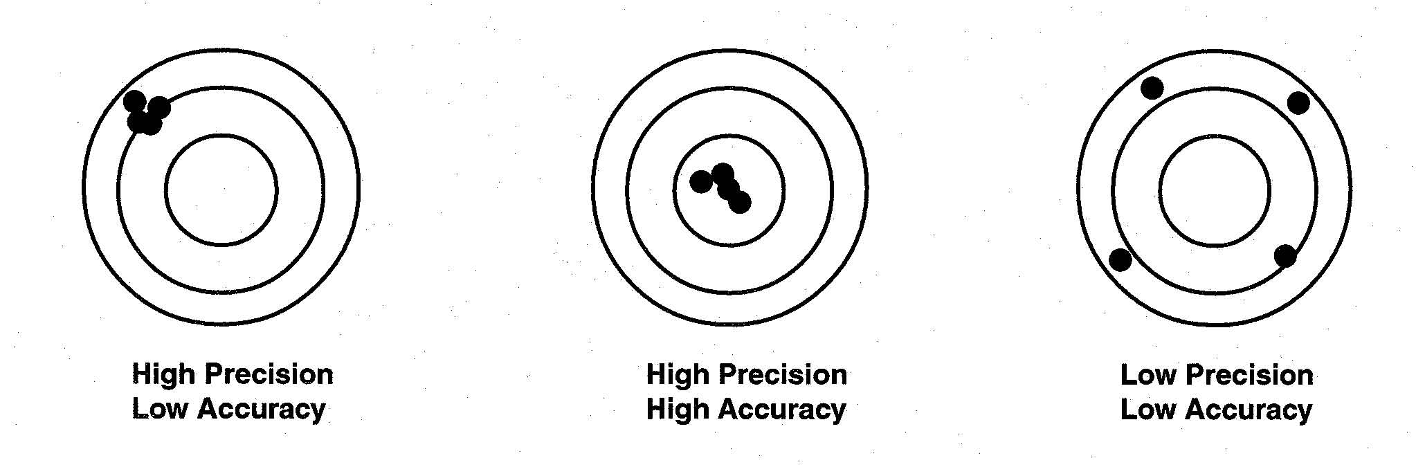
Definition of Precision and Accuracy

Psychometric arguments for out-of-level testing are that the scores will be more precise and accurate measures of student ability for those students who would otherwise earn very low scores on the grade level test. Classical test theory is founded on a test score model that assumes there are no perfect measures of ability. Each observed score (X) is comprised of that examinee’s true score (T) and a random error component (E):

Classical test theory refers to an individual’s expected score over repeated testing using the same (or equivalent test) as the examinees true score (Crocker & Algina, 1986). Random error is incorporated into the measurement model in order to account for the impact of fluctuations in testing conditions and examinee behavior that vary in unpredictable ways across occasions. Random error does not affect an examinee’s true score; rather it affects the consistency with which that score is estimated. Imagine a person who has no short-term memory repeatedly taking a test. His or her test score will vary across occasions – the greater the random error, the more variable the scores. Consistency or precision goes down as variability goes up. Reliability is a generic concept that is used as a barometer for the consistency or reproducibility of test scores.

Another type of error, known as systematic error represents error that consistently biases an examinee’s observed score in one direction. Systematic measurement errors do not result in imprecise (or inconsistent) measurement, but they result in less accurate measurement (Crocker & Algina, 1986). By accuracy, we are referring to the degree to which inferences from test scores are valid. We make the distinction between accuracy and precision to indicate that a test score can be highly precise or reliable, but not accurate or valid. The distinction is emphasized, in part, as a response to the over-emphasis placed on test score reliability in current research and discussions about out-of-level testing.

To further clarify the important conceptual distinction between precision and accuracy, we illustrate it with three simple diagrams. Each diagram in Figure 1 can be thought of as the possible scores an examinee could obtain on a test. Each dot represents the scores obtained from repeatedly testing the same person. The bulls-eye represents the person’s actual ability. We distinguish actual ability from true score; where true score represents an examinee’s expected score on those particular items – a concept that does not take into account that the items may be tainted by bias or that the items may not reflect those skills that the test purportedly measures.

In the first diagram, all four points lie in close proximity to each other, but to the left of the bulls-eye. This represents the case of high precision and low accuracy. The center of the four points represents the examinee’s true score. However, because all the points fell to the left of the bulls-eye, they are contaminated with systematic error, perhaps item bias, or inappropriate content to curriculum match. On the second bulls-eye, all four points lie in close proximity to each other, and all are inside the bulls-eye. This represents the case of high precision and high accuracy. In this illustration, the examinee’s true score and actual ability are very close. Such a test consists of unbiased items that represent the skills they purport to measure. On the third bulls-eye, the four points are distributed widely about the target. None of these points lies within the bulls-eye. This represents the case of low precision and low accuracy. These items may not have been well written – a factor that would likely affect the reliability and the validity of the scores.

Figure 1. Demonstration of How Random and Systematic Error Affect Precision and Accuracy

The diagrams illustrate three features of random and systematic error:

1. Random error affects precision, whereas systematic error affects accuracy.

2. A test score can be highly precise (reliable), without being accurate.

3. A test score cannot be highly accurate, unless it is highly precise.

 

Let’s assume that the Department of Transportation (DOT) in a certain state wants to determine how often people run the red light at a pre-selected highly traveled highway intersection. DOT places a sensor at the intersection that uses a laser to create an invisible line; when this line is crossed, it registers a single count in a computer, thus noting each time a car breaks through the line while the signal is red. The laser is active only while the traffic signal is red. DOT defines "running a red light" by any instance in which a car enters and proceeds through the intersection after the traffic light turned red. Let’s also assume that DOT is only interested in westbound traffic, and that it placed the camera at the far side of the intersection. Observations are made on five consecutive days, and the sensor runs 24 hours per day. Interest is in the expected number of times/day that cars run the red light.

Making daily counts over multiple days can be likened to repeatedly giving an examinee the same test. The average count across the five days can be likened to an examinee’s true score. Day-to-day fluctuations represent random error in estimating that value. The smaller the daily fluctuations, the more consistent are the day-to-day results, and thus, the more precisely the average count is estimated. Therefore, precision can be estimated directly from the observed counts.

One source of systematic error in this example comes from the placement of the sensor. Because the sensor is placed at the far end of the intersection, no cars that enter the intersection after the light turns red but turn left are counted. The result in that the actual number of cars running the red light is systematically underestimated. However, systematic error is not revealed directly from the data. Rather it stems from the inferences that are made from the observed data.

Imagine that DOT was conducting this study because a pedestrian walking across the highway 100 feet west of the intersection was struck by a car. After the incident many other reports surfaced about "near misses" that occurred when drivers ran the red light. Suppose, then, that DOT was only interested in counting cars that ran the red light and proceeded westbound on the highway. In other words, they were not interested in counting cars that ran the red light but turned left. In this case, the original placement of the sensor would not result in systematic underestimation of the true value; cars turning left no longer represent a source of systematic error. The point is that systematic error occurs, not through the data alone, but from inferences based on the data.

The DOT example also demonstrates another feature of systematic error: a score can be precisely measured while not being accurately measured. If it happens that the day-to-day fluctuations in cars counted were very small, then each daily count would be very close to the mean of the counts across days (true score), and DOT’s counts would represent a precise estimate. However, if many cars turned left after entering the intersection on a red light, and interest was in all cars running the red light, then DOT’s count of the number running the red light would grossly underestimate the actual count; the estimate would be inaccurate. Such instances of precise, but inaccurate measures may be a common occurrence in achievement testing, a field in which measurement precision is a primary concern.

Out-of-level Testing and Measurement Precision

Empirical studies of how out-of-level testing affects test scores have primarily used two criteria for describing and interpreting the effects: internal consistency reliability and the percent of test scores at or above chance level – the latter representing a proxy for the former. The popularity of these criteria has more to do with their familiarity and the ease with which they can be calculated than with a strong psychometric foundation. To be sure, both concepts loosely gauge the precision with which individual test scores are measured, but neither method reveals a direct link to precision.

The concept of reliability was derived from classical test score theory as a means of indexing random measurement error. Reliability is better described as an index of how much of the variability in a set of test scores represents true score variation. Reliability provides information about measurement precision for a group of test scores, but it is a poor and often misleading gauge of the precision of a particular score.

Reliability indices reported by most test publishers come from a class of methods known as internal consistency methods because they estimate how consistently examinees perform across items. The stronger the correlation between performance on one item and performance on other items for a group of examinees, the higher the reliability index. All examinees contribute equally to test score reliability. A test would be perfectly reliable if all examinees with the same test score had the same performance pattern across items. Because most test scores lie near the group mean, the internal consistency index is influenced more by scores at or near the mean than by scores at either extreme. Therefore, when we say a test is reliable, we mean that it is reliable for examinees earning scores near the middle of the test score distribution. Scores falling at the tails of the test score distribution may not be reliable.

There are other reasons why reliability is an inadequate index of test score quality. Reliability is affected by the characteristics of the particular sample upon which it was measured. Change the sample and you change the reliability. For instance, if the range of scores in a sample is small, then it does not matter what percent lie above chance, the reliability index will be low. More important, is that using a single reliability index implies that measurement precision is a constant across ability levels. If this were true, there would be no need for out-of-level-testing.

It has been understood for some time that measurement error varies systematically with test score. If one were to plot a graph of measurement error on the y-axis and test score along the x-axis, the curve would be U-shaped, with high measurement error at the test score extremes and low measurement error near the middle. An important goal of out-of-level testing is to decrease the measurement error for examinees at the test score extremes. The general idea is that if you give a low scoring examinee an easier (lower level of a test) the examinee’s test score on the easier test will lie closer to the middle of the x-axis, the point where the U-curve is lowest. Unfortunately, the relationship between measurement error and test performance cannot be demonstrated with classical test score theory concepts so familiar to most practitioners. In order to demonstrate the relationship we need to draw on concepts from a theory of scaling tests known as item response theory (IRT).

IRT Informs Precision

Item response theory is represented by a set of mathematical models that relate the probability that an examinee will correctly answer an item to certain characteristics of the item and the examinee (Hambleton & Swaminathan, 1995). The most basic IRT model is called the Rasch model after Georg Rasch who developed the foundational work on the model (Rasch, 1960). The Rasch model states that, for a randomly selected person with a certain ability, referred to as "theta," the probability of a correct response to item j depends only on the difficulty of the item. This is presented in the following formula:

In this formula, q represents the ability of the examinee i, b represents the difficulty of item j, and D is a constant. When integrated over the ability continuum, this function forms a curve called the item characteristic curve. With IRT, person ability and item difficulty are estimated on the same scale. For simplicity, this scale is constrained to have a mean equal to zero and a standard deviation equal to 1.0. In this way, it is similar in form to the z-score scale.

Figure 2 shows a hypothetical item characteristic curve. The x-axis represents the scale along which item difficulty and person ability are measured. It is reasonable to constrain the bounds of this scale to ± 3 standard deviation units (99.5% of the population will fall within these bounds). Every examinee represents a single point defining this curve. Using the Rasch model, item difficulty is defined as the point on the x-axis that corresponds to the value of .50 on the y-axis, in other words, a 50% chance of getting the item correct. For this item, the difficulty was -.41.

Figure 2. Item Characteristic Curve and the Associated Item Information Function for an Item with a Difficulty Equal to -.41

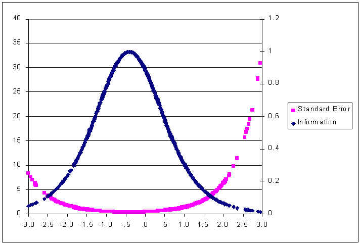
The figure shows that the probability of getting an item correct increases as person ability (qi) increases with respect to item difficulty (bj). The curve relating examinee ability and the probability of getting the item correct is "S" shaped. Across a broad range of ability, the curve forms a straight line, but at either end, it flattens. The flattened regions represent the ability range at which the item does not discriminate very well. A substantial change in ability corresponds to only a very small change in the probability of getting the item correct. For example, an examinee with ability equal to 1.6 has a 97% chance of getting the item correct; whereas an examinee with an ability of 2.1 (one-half of a SD higher) has a 98% chance of getting the item correct. The item does not differentiate very well between these ability levels. On the other hand, a one-half of a standard deviation unit difference in ability in the range between -.5 and 0.0 results in a substantial change in the probability of passing the item. An examinee with an ability equal to -.5 has roughly a 44% chance to pass the item, whereas an examinee with an ability one-half a standard deviation unit higher, 0.0, has roughly a 66% chance of passing the item. Across an equally sized interval, the probability of passing this particular item changes more dramatically for examinees whose ability falls between -1.0 and .50, than it does outside this range. We say that the item provides more information about examinees whose ability falls along the steep range of the curve than it does for examinees whose ability falls in the range where the curve becomes flat.

Item information is directly proportional to the square of the slope of the item characteristic curve. The function peaks (denotes most information) precisely at the point corresponding to the item’s difficulty. In Figure 2, the peak of the item information function corresponds precisely to the difficulty of the item. An important feature of item information functions is that they can be summed in order to generate an information function for an entire test. Because these functions can be summed, and because the peak of each corresponds to its difficulty, then a simple histogram of the item difficulties can be used to indicate the range across which the test is most informative. The test is most informative across the ability levels corresponding to the difficulty levels where most items lie. The reason why scores at the extremes are not very precise is that there are few very easy and very hard items to provide information about examinees at these levels.

To understand the importance of the distribution of item difficulties, imagine that we have a five-item test wherein all items have the same difficulty as the item shown in Figure 2. The information function for all five items, called the test information function, could be estimated by multiplying the value of the information function at each point on the ability scale by five. The information at all ability levels would increase, but the information for scores corresponding to ability near -.41 (see Figure 2) would increase dramatically. The result would be a curve that looks just like the curve in Figure 3, with the exception that the curve would be much more peaked. The test would be extremely informative across a narrow ability range centered at -.41.

The downside of talking about the information function is that its scale has little meaning for most practitioners. A concept that resonates more with practitioners is the standard error of measurement (described above). In IRT, there is an inverse relationship between the conditional standard error of measurement and the information function; the standard error of ability estimation is lowest for the ability that corresponds to the peak of the item information function. As in classical test score theory, the standard error of measurement can be used to create confidence intervals around an observed score in order to determine the range within which the examinee’s true score lies.

Figure 3 is an example of the test information function from an actual test, the 1988 National Educational Longitudinal Study (NELS:88) mathematics test. The test was a 40-item multiple-choice test. In many ways the NELS:88 math test mirrors NRTs. It uses multiple-choice items, it has a similar number of items, and its primary purpose was to provide accurate measurement of the status of individuals at a given point in time, as well as growth over time (Spencer et al., 1990).

Figure 3. Test Information Function and Standard Error of Measurement for the NELS:88 Base Year Mathematics Test

Norm-referenced tests are designed to maximize test information for the majority of the examinees. Because ability is assumed to form a normal distribution, most examinees fall within ± 1 standard deviation from the mean. To maximize information for this group of examinees, test publishers select items so that the distribution of item difficulty is also normal, with a mean equal to the mean of the population’s ability. The result is a test that is informative for the 84% of the examinees whose ability falls within ± 1 standard deviation of the population mean.

The range over which one would say that a test is reliable depends on how much measurement error is deemed acceptable. Measurement precision for an achievement test is usually considered acceptable when the reliability index exceeds .85. Using the relation from classical test theory between test reliability and measurement error (i.e., error = SD * sqrt (1 - r_xx), a reliability of .85 would imply that one is willing to consider a person’s test score to be reasonably reliable when the measurement error on that score falls below .39 x SD (where sqrt 1 - .85 = .39). Under IRT parameterization, test performance is scaled to have a standard deviation equal to 1.0. Therefore, measurement error for an individual would be acceptable if it was below .39. The right side axis on Figure 3 indicates the amount of measurement error contained in a score at each ability level. If we drew a horizontal line from the right axis at a value of .39 until it crossed the SE curve and then drew a vertical line down to the x-axis, we would obtain an upper limit for reliable performance corresponding to "theta"=1.7. Repeating this procedure to get the lower bound we would find it to be -1.0. In other words, only those examinees whose performance fell within the range -1.0 and 1.7 would have a reasonably reliable measure of performance. The standard error for a very low performing examinee, for example one whose ability estimate is more than two standard deviations below the mean would be unacceptably high. For instance, the 95% confidence interval for an examinee with an ability estimate of -2.5 would range from –4.5 to -0.5. In other words, the best one could say is that that examinee’s true performance lies somewhere between very low and average ability. Obviously, this is a rather crude estimate of ability. On the other hand, the 95% confidence band for an examinee performing at the mean (x=20) would range from -.3 to .7. We can say with certainty that, with respect to the norm group, this individual is of average ability.

This is the situation with most norm-referenced tests. In order to get a more precise ability estimate for low ability examinees the test would need many more easy items, items that provide information for low performing examinees. An alternative method would be to give these students an easier version of the test, so that their performance places them nearer to the middle of the score distribution—the place where the test is most precise. This is what out-of-level testing attempts to accomplish.

To illustrate how out-of-level testing can be used to increase measurement precision, we present the conditional standard error of measurement curves for two tests of the same length but of different difficulty (see Figure 4). The x-axis represents the ability/difficulty scale. Recall that with IRT, ability and item difficulty are estimated on the same scale. The out-of-level test has an average difficulty level of 0.0, whereas the in-level test has an average difficulty level of .50. An average difficulty difference of .50 standard deviation units is similar to the difference found between adjacent levels of many NRTs. If an examinee with ability equal to –2.0 (i.e., 2 standard deviations below the population mean) took the in-level test, his or her standard error of measurement would be about 1.5. The 95% confidence bands on that examinee’s score would range between -5.0 to +1.0 on the in-level test. However, if that same examinee took the out-of-level test, his or her standard error would be about .50, with the true range between -3.0 to -1.0 using the out-of-level test. Clearly, the out-of-level-test provides a far more precise estimate of that examinee’s ability than the in-level test. In fact, whenever two different levels of a test have a high content alignment, and item difficulty is normally distributed on both levels, the lower level test will result in more precise ability estimation for the very low performing examinees. Psychometric theory tells us that this must be the case. No empirical studies are required to establish this fact. Since most NRTs satisfy both requirements, we can safely assume (without the need for empirical investigation) that test performance on an out-of-level test will result in more precise measurement for low performing examinees.

Figure 4. Standard Error of Measurement for Two Hypothetical Tests that Differ in Their Average Difficulty Level

Precise measurement on the out-of-level-test does not ensure that the score accurately reflects the performance that would be obtained on the in-level test. Somehow, the score from the out-of-level test must be converted into a score on the in-level test. The method for converting scores from one level of a test onto the scale of another level is known as vertical equating. A tenet of vertical equating is that the examinee should obtain the same proficiency estimate regardless of the particular level of the test he or she takes. If this tenet is satisfied then the result is increased measurement precision for low ability examinees, along with a score that can be directly interpreted with scores obtained on examinees taking the grade level test. This result should bring euphoria to those who are required to include students with disabilities in the same assessment system as their non-disabled peers, and who desire to draw meaningful comparisons between the groups. Instead of having quality scores for roughly 80% of the students, they can have quality scores, without the need for separate testing systems on as much as 98% of the students. However, the euphoria may be overstated, or premature. Vertical equating necessarily introduces some measurement error, and it may introduce bias (Kim & Cohen, 1998).

Through a series of equating studies and relying on the tenets of item response theory, test publishers have created scales that span the full spectrum of their achievement tests from elementary school through high school. They refer to this as vertical scaling. Scores for students taking different levels are all reported on a single scale. For instance, the score for a 4th grader taking the 4th grade level of the ninth edition of the Stanford Achievement Test (SAT-9) is reported on the same scale as the score for a 7th grader taking the 7th grade SAT-9. Likewise, the score of a 7th grader taking the 6th grade test is reported on the same scale as other 7th graders taking the 7th grade test. The primary purpose for creating a single scale was to permit test users, such as school districts, a better means of tracking achievement growth across years and grades. Another benefit of forming a single scale that spans all levels of the test, a benefit that is relevant to out-of-level-testing, is that an examinee’s position along the scale should not be dependent on the particular level of the test that he or she takes. Whether a student takes the grade level test, or a test one or two levels below, the scale score is on the same scale, and therefore can be compared to the scaled score of examinees taking the grade level test. No further equating is required. The question becomes, how much error is added to score estimates as a result of vertical equating?

There are many methods available to test publishers to conduct vertical equating studies, each with its own set of assumptions. Describing all of the methods of vertical equating is beyond the scope of this paper; the reader is referred to the Holland and Rubin (1985). Our discussion will focus on one method of vertical equating in which IRT is used to simultaneously generate item difficulty estimates across two levels of the test.

A minimum requirement to conduct equating is that the two tests measure the same ability. To this end, test publishers select test items so that adjacent levels of the tests overlap in both content and skills. Despite this overlap, there is reason to believe that different levels of a test may not satisfy the assumption that each measures the same ability (Yen, 1985). A second requirement is that either a common set of examinees takes both tests, called the single group design, or there is a common set of items appearing on both tests, called the anchor test design (Hambleton & Swaminathan, 1995). A bonus of using the anchor test design is that the participants are not required to take both tests, thus eliminating fatigue effects. Additionally, neither the examinees nor the tests need to be equivalent. That is why it lends itself well to vertical equating studies (Vale, 1986). An increasingly popular approach to vertical equating is to concurrently calibrate the pool of items across both groups of examinees. IRT programs such as BILOG-MG (Zimowski, Muraki, Miselvy, & Bock, 1996) and MULTILOG (Thissen, 1991) can concurrently calibrate items appearing on different tests and administered to different examinees, provided a common core of items is taken by all examinees. When calibrated concurrently, the item difficulties and the person abilities are on a common scale.

The first step for concurrent calibration of test items is to choose one level of the test, usually one near the middle of the continuum (e.g., the 6th test) as the anchor test. The anchor test is used to determine the unit of the scale (i.e., the standard deviation), and to fix the origin. The origin is defined as the mean difficulty level of the anchor test. Once the anchor test is chosen, that test and an adjacent test (one level below or one level above) are administered to a sample of students at the grade level corresponding to the grade level of the anchor test. All items from both tests are analyzed together using an IRT model of the test publisher’s choice.

The way to get the items from the remaining tests onto the same scale as the 6th grade anchor test is to repeat this process with pairs of tests at each adjacent level, and to determine an equating constant for each level of the test. For example, let’s assume that the first calibration was done by administering to a sample of 6th graders both the 6th grade and 5th grade test. The next step would be to give a sample of 5th graders both the 5th grade and 4th grade test, and treat these items as though they represented a single test. Again, the result is that the item difficulty estimates for the 4th and 5th grade test items are on a common scale. However, they are not yet on the scale defined by the 6th grade test. We have two pools of items (4th/5th grade items, and 5th/6th grade items) given to two different populations; 5th graders and 6th graders. The items can be linked because there is a subset of items, namely the 5th grade test items that were used in both calibrations. These items are called the "linking items." Now, it is only a matter of determining the appropriate equating constant. The reason why an equating constant is necessary has to do with the fact that item parameters derived from IRT models are only invariant up to a linear transformation. Provided that all the items from two different tests measure a single trait, and the IRT model fits the data, the two sets of item parameter estimates obtained on the same set of items, using two different groups of examinees, should be linearly related.

If a scatter-plot was made, the item difficulty estimates should all fall on a line with slope equal to 1.0. In order to place the items onto a common scale, we need only to determine the appropriate equating constant. Using the Rasch model to estimate item parameters, the separate calibrations of each test produce a pair of independent item difficulties for each linking item. In our example, the 5th grade test items represent the linking items, because they were calibrated separately using 5th graders and 6th graders. According to the model, the estimates of each pair are statistically equivalent except for a single constant of translation common to all pairs in the link. When two tests, A and B are joined by a common link of k items, and each test is given to a different sample, and biA and biB are estimated item difficulties of item i in each test, the single constant necessary to translate all item difficulties in the calibration of test B onto the scale of test A (Wright & Stone, 1979) is described by the following formula:

In this formula, EC stands for equating constant. In our example, test A represents the simultaneous calibration of the 5th grade and 6th grade test items on the 6th grade sample, and test B represents the simultaneous calibration of the 4th and 5th grade test items on the 5th grade sample. The 5th grade test items are the k linking items. Subtracting the equating constant, EC, from the item difficulty estimates of the 4th grade test items places those items onto the metric of the anchor test. These steps are repeated for all adjacent levels of the test until all item difficulty estimates are on a common metric. Once the calibration of all items is complete, the item difficulty estimates are treated as known values and they are fixed for the calibration of person ability.

In order to understand how the equating introduces error, we introduce a statistic called the root mean square error (RMSE). In the present vertical equating procedure using the Rasch model, the RMSE can be defined as:

In this formula EC represents the equating constant and other values are defined as they are in the previous equation. When all pairs of item difficulty estimates fall on a line, the RMSE will equal zero. A RMSE greater than zero indicates that the equating method introduced error, which subsequently reduces the precision of measurement of an examinee’s scaled score. In addition to the error introduced in the linking procedure, simultaneous calibration of item parameters also introduces some error. However, Kim and Cohen (1998) found that when the number of items is sufficiently large (N=50), simultaneous calibration resulted in about the same amount of error as separate item calibration. Perhaps more important to our discussion of measurement error and out-of-level-testing, Cohen and Kim stated that the evaluation of the accuracy of linking can only be accomplished with simulation studies, because there is no criterion with which to evaluate the accuracy of the results.

It is incumbent on test publishers to demonstrate that the assumptions of their equating model are met, and to show the amount of equating error. Unfortunately, our examination of technical reports made available by several test publishers (see Bielinski, Scott, Minnema, & Thurlow, 2000) indicated that the reports do not include the necessary data. This practice is likely to change, however, because the latest edition of the Standards for Educational and Psychological Testing (APA/AERA/NCME, 1999) states that test publishers should provide detailed technical information on the method by which equating functions were established and on the accuracy of equating functions (Standard 4.11, p. 57). The standard further states, "The fundamental concern is to show that equated scores measure essentially the same construct, with very similar levels of reliability and conditional standard errors of measurement" (APA/AERA/NCME, 1999, p. 57). The challenge for out-of-level-testing research is to demonstrate that the gain in precision obtained by giving the student a test other than the one developed for his or her grade level far outweighs the loss in precision due to test score equating. The void in our knowledge of the measurement error that is introduced by equating represents an important drawback to its use.

Test Score Accuracy

A fundamental issue for out-of-level testing is whether its use results in more or less accurate scores than in-level testing. Proponents of out-of-level testing state that it increases accuracy by reducing guessing and eliminating floor effects. Both of these factors, when present, may bias grade test scores upward for low achieving students. Proponents also argue that the content and skills measured by an out-of-level test may better match an examinee’s classroom instruction. Opponents suggest that out-of-level testing decreases accuracy because the out-of-level test does not align to the standard they are measuring, or because test score equating necessarily introduces bias.

Both of the above arguments may be correct. The validity of out-of-level test scores depends, in part, on the intended use of the test score. When test scores are used to determine proficiency with respect to content or process standards that are linked to grade level, as is the case with high stakes testing for graduation or district accountability, then out-of-level testing would be inappropriate. The reason is that out-of-level test items tap different content and measure different skills than the grade level tests; prediction of performance cannot be made on content or skills beyond those measured by the test that is taken. In other words, one cannot say anything about how a student will do on algebra items based on the student’s performance on computation items. On the other hand, when the purpose is to determine proficiency in a content domain, or to track achievement growth, then out-of-level testing may be appropriate. Even when out-of-level-testing is appropriate, claims of increased accuracy must still be demonstrated. This will require that validity studies be conducted in which scores from out-of-level tests are correlated with other reliable measures of the skills purportedly measured by that test.

Guessing Affects Accuracy

A principal claim of proponents of out-of-level testing is that its use may reduce guessing. Guessing represents a form of systematic error wherein an examinee’s score is biased upward. All multiple-choice test scores can be affected by guessing, but the claim by out-of-level testing proponents appears to be that low performing examinees guess more than other examinees. If scores for low performing students are more contaminated by guessing than scores for other students, then the size of the gap between low and moderate performing students is artificially reduced, and one may conclude that low performing examinees have more proficiency than they actually have. Additionally, it is more difficult to detect proficiency gains in scores contaminated by guessing. The presence of guessing may be a double-edged sword; proficiency will be overstated, and real gains will go unnoticed. The detrimental effects of guessing may be mitigated by methods that adjust for differential guessing.

Methods have been developed to adjust for random guessing. Methods based on raw scores are commonly referred to as formula scoring (Crocker & Algina, 1986, p. 401). All formula scoring methods assume that guessing is random. For instance, the "rights minus wrongs" correction subtracts from a person’s obtained score the number the person got wrong divided by the number of alternatives minus 1. This is represented in the following formula:

The assumption is that each incorrect response is the result of a random guess. Dividing the number wrong (W) by k-1 yields an estimate of the number of items that the examinee probably answered correctly by guessing. This quantity is subtracted from the examinee’s obtained score to correct for guessing. An item response theory model, known as the three-parameter logistic model, includes a parameter that adjusts ability estimates for guessing (Hambleton & Swaminathan, 1995). Even though these adjustments have been made, studies on out-of-level testing still neglect the possibility that such corrections for guessing may be sufficient to increase test score accuracy.

Implied, but seldom stated by proponents of out-of-level testing, is that examinees who earn scores at or below chance level guess more often than high performing examinees. This belief is so deeply entrenched in the minds of some proponents, that, without reference to supporting literature, the reduction of the number of chance level scores has become a hallmark for demonstrating the effectiveness of out-of-level-testing (Ayrer & McNamara, 1973; Cleland, Crowder, 1978; Easton & Washington, 1982; Howes, 1985; Jones et al., 1983; Powers & Gallas, 1978; Slaughter & Gallas, 1978; Winston, & Idstein, 1980; Yoshida, 1976). It is as though chance level scoring necessarily indicates random guessing. We know of no study that definitively demonstrates that chance level scores are obtained solely by guessing. Nor are there studies that show scores at or below chance are contaminated more by guessing than any other score. Rather, low performing examinees are likely to omit more items, in which case their performance, uncorrected for guessing, will be underestimated (Lord, 1975).

Several studies found that the proportion of chance level scores decreases when low performing examinees (often defined by those scores at or below chance level) take a lower level of the test (Ayrer & McNamara, 1973; Crowder, 1978; Easton & Washington, 1982). In these studies all participants were administered the in-level test and another test at least one level below. In other studies, results indicate that these students may have to go down more than one level in order to observe a substantial decrease in the number of chance scores (Cleland, Winston, & Idstein, 1980; Jones et al., 1983; Slaughter, Helen, & Gallas, 1978). Unfortunately, the curriculum overlap may be too sparse to obtain comparable information when more then one level below grade level is used.

A shortcoming to many of these studies is that they excluded high performing examinees. It may very well be that the scores of high performing examinees also decrease when an out-of-level-test is used. There is some confirmation of this in the literature. In a study by Slaughter (1978), students who took both an in-level and an out-of-level-test were divided into three groups based on their performance on the in-level test: (1) those scoring near the floor, (2) those scoring between floor and ceiling, and (3) those scoring at or above the ceiling. All students took the in-level test, and half took the adjacent lower level, while the other half took the test two levels below. Scores were reported on a common metric so the differences between scores on the grade level and out-of-level-test could be computed. The difference scores between the grade level and the adjacent lower level were, on average, of the same magnitude across groups. Given the direction of the difference score, it appeared that scores dropped for all groups. None of the difference scores was significant. The difference scores between the in-level test and the test two levels below varied across groups. The "floor" group showed a statistically significant drop, whereas the other two groups showed drops of about the same magnitude as in the first comparison. Those who insist that guessing contaminates scores more for the floor group could use these results to support their contention. On the other hand, the data demonstrate that all scores drop regardless of the performance level. By giving only the low performing students the out-of-level test, one is artificially increasing the gap between them and higher performing students.

The primary purpose of out-of-level testing is to increase measurement precision and test score accuracy for students who score at the test score extremes on the grade level test. Studies of out-of-level testing traditionally rely on classical test theory notions of measurement precision, particularly test score reliability. Reliability obscures the true nature of how it is that an out-of-level test increases measurement precision. Using item response theory, it can be shown that scores at the extremes contain more error (i.e., are less precise) because there are fewer items available to discriminate between examinees at very low or very high ability levels. The relationship between examinee ability and test score precision derives directly from the mathematics of IRT; further empirical evidence is not necessary. That tests are less precise at the test score extremes is built in by design. Test publishers must balance high quality measurement with practical limits on the number of items on a test.

Vertical scaling makes it possible to obtain meaningful scores on out-of-level tests. Unfortunately, the process introduces a certain amount of measurement error. To date, there are no data available from test publishers as to how much error is introduced by their vertical scaling methods. Because the new testing standards recommend that test publishers include information on equating error, we expect this situation to change in the near future.

Proponents of out-of-level testing claim that it improves measurement precision as well as test score accuracy. The claim is premised on the belief that low scoring students guess more than other students, and that when the examinee takes items better suited to his or her ability, motivation for guessing will drop. Support for this assumption is sketchy at best. Besides, scaled scores are determined by IRT models that often employ a parameter that adjusts the score for guessing. More validity studies are needed to demonstrate improvement in test score accuracy.

American Psychological Association, American Educational Research Association, & National Council on Measurement in Education. (1999). Standards for educational and psychological testing. Washington, DC: American Psychological Association.

Arter, J. A. (1982, March). Out-of-level versus in-level testing: When should we recommend each? Paper presented at the annual meeting of the American Educational Research Association, New York, NY.

Ayrer, J. E. & McNamara, T. C. (1973). Survey testing on an out-of-level basis. Journal of Educational Measurement, 10 (2), 79-84.

Bejar, I. I., Weiss, D. J. & Gialluca, K. A. (1977). An information comparison of conventional and adaptive tests in the measurement of classroom achievement. (Research Report 77-7). Minneapolis. University of Minnesota, Psychometric Methods Program, Department of Psychology.

Bielinski, J., Scott, J., Minnema, J., & Thurlow, M. (2000). Test publishers’ views on out-of-level testing (Out-of-Level Assessment Report 3). Minneapolis: University of Minnesota, National Center on Educational Outcomes.

Clarke, M. (1983, November). Functional level testing decision points and suggestions to innovators. Paper presented at the meeting of the California Educational Research Association, Los Angeles, CA.

Cleland, W. E. & Idstein, P. M. (1980, April). In-level versus out-of-level testing of sixth grade special education students. Paper presented at the annual meeting of the National Council on Measurement in Education, Boston, MA.

Crocker, L., & Algina, J. (1986). Introduction to classical and modern test theory. Chicago, IL: Holt, Rhinehart, and Winston Inc.

Crowder, C. R., & Gallas, E. J. (1978, March). Relation of out-of-level testing to ceiling and floor effects on third and fifth grade students. Paper presented at the annual meeting of the American Educational Research Association, Toronto, Ontario, Canada.

Easton, J. A., & Washington, E. D. (1982, March). The effects of functional level testing on five new standardized reading achievement tests. Paper presented at the annual meeting of the American Educational Research Association, New York, NY.

Haenn, J. F., & Proctor, D. C. (1978, March). A practitioner’s guide to out-of-level testing. Paper presented at the annual meeting of the American Educational Research Association, Toronto, Ontario, Canada.

Haenn, J. F. (1981, March). A practitioner’s guide to functional level testing. Paper presented at the annual meeting of the American Educational Research Association, Los Angeles, CA.

Hambleton, R. K., & Swaminathan, H. (1995). Item response theory: Principles and applications. Boston, MA: Kluwer Nijhoff.

Haynes, L. T., & Cole, N. S. (1982, March). Testing some assumptions about on-level versus out-of-level achievement testing. Paper presented at the annual meeting of the National Council on Measurement in Education, New York, NY.

Holland, P. W., & Rubin, D. B. (Eds.). (1985). Test equating. New York, NY: Academic Press.

Howes, A. C. (1985, April). Evaluating the validity of Chapter I data: Taking a closer look. Paper presented at the annual meeting of the American Educational Research Association, Chicago, IL.

Jones, E. D., Barnette, J. J., & Callahan, C. M. (1983, April). Out-of-level testing for special education students with mild learning handicaps. Paper presented at the annual meeting of the American Educational Research Association, Montreal, Quebec.

Kim, S-H., & Cohen, A. S. (1988). A comparison of linking and concurrent calibration under item response theory. Applied Psychological Measurement, 22 (2), 131-143.

Long, J. V., Schaffran, J. A., & Kellogg, T. M. (1977). Effects of out-of-level survey testing on reading achievement scores of Title I ESEA students. Journal of Educational Measurement, 14, (3), 203-213.

Lord, F. M. (1975). Formula scoring and number-right scoring. Journal of Educational Measurement, 12 (1), 7-11.

McBride, J. R. (1979). Adaptive mental testing: The state of the art (Report No. ARI-TR-423). Alexandria, VA: Army Research Institute for the Behavioral and Social Sciences. (ERIC Document Reproduction Service No. ED 200 612).

Minnema, J., Thurlow, M., Bielinski, J., & Scott, J. (2000). Past and present understandings of out-of-level testing: A research synthesis (Out-of-Level Testing Report 1). Minneapolis: University of Minnesota, National Center on Educational Outcomes.

Plake, B. S., & Hoover, H. D. (1979). The comparability of equal raw scores obtained from in-level and out-of-level testing: One source of the discrepancy between in-level and out-of-level grade equivalent scores. Journal of Educational Measurement, 16 (4), 271-278.

Psychological Corporation, Harcourt Brace & Company (1993). Metropolitan Achievement Tests, Seventh Edition. San Antonio, TX: Author.

Psychological Corporation, Harcourt Brace Educational Measurement (1997). Stanford Achievement Test Series, Ninth Edition. San Antonio, TX: Author.

Rasch, G. (1960). Probabilistic models for some intelligence and attainment tests. Copenhagen: Danish Institute Educational Research.

Roberts, A. (1976). Out-of-level testing. ESEA Title I evaluation and reporting system (Technical Paper No. 6). Mountain View, CA: RMC Research Corporation.

Rudner, L. M. (1978, March). A short and simple introduction to tailored testing. Paper presented at the annual meeting of the Eastern Educational Research Association, Williamsburg, VA.

Slaughter, H. B., & Gallas, E. J. (1978, March). Will out-of-level norm-referenced testing improve the selection of program participants and the diagnosis of reading comprehension in ESEA Title I programs? Paper presented at the annual meeting of the American Educational Research Association, Toronto, Ontario, Canada.

Smith, L. L., & Johns, J. L. (1984). A study of the effects of out-of-level testing with poor readers in the intermediate grades. Reading Psychology: An International Quarterly (5), 139-143.

Spencer, B. D., Frankel, M. R., Ingels, S. J., Rasinski, K. A., & Tourangeau, R. (1990). National Educational Longitudinal Study of 1988: Base year sample design report. NCES Report 90-463. Washington, DC: National Center for Education Statistics.

Thissen, D. (1991). MULTILOG user’s guide. Scientific Software Inc.

Thurlow, M., Elliott, J., & Ysseldyke, J. (1999). Out-of-level testing: Pros and cons (Policy Directions 9). Minneapolis: University of Minnesota, National Center on Educational Outcomes.

Vale, C. D. (1986). Linking item parameters onto a common scale. Applied Psychological Measurement, 10(4), 333-344.

Wheeler, P. H. (1995). Functional-level testing: A must for valid and accurate assessment results. (EREAPA Publication Series No. 95-2). Livermore, CA: (ERIC Document Reproduction Service No. ED 393 915)

Wick, J. W. (1983). Reducing proportion of chance scores in inner-city standardized testing results: Impact on average scores. American Educational Research Journal, 20 (3), 461-463.

Wilson, K. M., & Donlon, T. F. (1980). Toward functional criteria for functional-level testing in Title I evaluation. New Directions for Testing and Measurement, 8, 33-50.

Wright, B. D., & Stone, M. H. (1979). Best test design: Rasch measurement. Chicago, IL: Mesa Press.

Yen, W. M. (1985). Increasing item complexity: A possible cause of scale shrinkage for unidimensional item response theory. Psychometrika, 50(4), 399-410.

Yoshida, R. K. (1976). Out-of-level testing of special education students with a standardized achievement batter. Journal of Educational Measurement, 13 (3), 215-221.

Zimowski, M. F., Muraki, E., Mislevy, R. J., & Bock, D. R. (1996). BILOG-MG: Multiple-group IRT analysis and test maintenance for binary items. SSI Scientific Software Inc.

  Top of page